1. Interpreting hidden representations
1.1 Invertible transformation of hidden representations

- Input image: \( x \in \mathbb{R}^{H \times W \times 3 } \)
- Sub-network of \(f \) including hidden layers: \(E\)
- Latent (original) representation: \( z=\mathbb{E} (x) \in \mathbb{R}^{H \times W \times 3 = N}\)
- Sub-network after the hidden layer: \( G \)
- \( f(x)=G \cdot E(x) \)
In A Disentangling Invertible Interpretation Network for Explaining Latent Representations, the goal is to translate an original representation \(z\) to an equivalent yet interpretable one.
In order to \(z\) into an interpretable representation, the following is introduced.

So, what can we obtain from interpretable representations??
(i) We can comprehend the meaning of the latent variable from the value of interpretable representation and get more natural images from GAN.

(ii) Semantic image modifications and embeddings. As we manipulate the semantic factor (=interpretable representation) for digit, we can get '3' digit image from '9' digit image.

1.2 Distangling interpretable concepts
What properties of \( \widetilde{z}_k \) we should satisfy??
A. It must represent a specific interpretable concept. (ex: color, class ...)
B. It is independent of each other.
\( \quad \Rightarrow P(\widetilde{z})=\Pi^K P(\widetilde{z}_k) \)
C. Distribution \( P(z_k) \) of each factor must be easy to sample from to gain insights into the variability of a factor.
D. Interpolation between two samples of a factor must be valid samples to analyze changes along a path
Satisfy C. and D. \( \Rightarrow \) \( P(\widetilde{z})=\Pi^K N(P(\widetilde{z}_k | 0,1) \quad \cdots Eq. (1) \)
The way to supply additional constraints for Eq. (1).
Let there be training image pairs \( (x^a x^b) \) which specify semantics through their similarity.
Each semantic concept \( F \in \{ 1, \cdots , K \} \) defined by such pairs is represented by corresponding factor \( \widetilde{z}_F \) and we write \( (x^a, x^b) \sim P(x^a,x^b|F) \) to emphasize that \( (x^a,x^b) \) is a training pair for factor \( \widetilde{z}_F \).
However, we cannot expect to have examples of image pairs for every semantic concept relevant in \( z\).
\( \quad \Rightarrow \) So, let introduce \( z_0 \) to act as a residual concept
For a given training pair \( (x^a, x^b) \) factorized representation \( \tilde{z}^a=T(X(x^a)) \) and \( \tilde{z}^b=T(X(x^b)) \) must \( (i) \) mirror the semantic similarity of \((x^a, x^b) \) in its \(F\)-th factor and \( (ii) \) be invariant in the remaining factors.
\( \quad (i) \) a positive correlation factor \( \sigma_{ab} \in (0,1) \) for the \(F\)-th factors between pairs
\( \quad \quad \Rightarrow \) \( \widetilde{z}^b_F \sim N (\widetilde{z}^b_F | \sigma_{ab} \widetilde{z}^a_F , (1- \sigma_{ab} ) \mathbf{1} ) \quad \cdots Eq. (2) \)
\( \quad (ii) \) no correlation for the remaining factors between pairs
\( \quad \quad \Rightarrow\) \( \widetilde{z}^b_k \sim N (\widetilde{z}^b_k | 0,1 ) ; k \in \{ 0, \cdots , K \} \backslash \{ F \} \quad \cdots Eq. (3) \)

To fit this model to data, we utilize the invertibility of \(T\) to directly compute and maximize the likelihood \( (z^a, z^b)=(E(x^a), E(x^b)) \).
Compute the likelihood with the absolute value of the Jacobian determinant of \(T \), denoted \(T'(\cdot)\), as

Build \(T\) based on ActNorm, AffineCoupling, and shuffling layers. (detailed in an original paper...)
For training, we use negative log-likelihood as our loss function.
Subsitituting Eq. (1) into Eq. (4), Eq. (2) and (3) into Eq.(5) leads to the per-example loss \(l(z^a,z^b |F)\).

The loss function is optimized over training pairs \( (x^a, x^b) \) for all semantic concepts \( F \in \{1, \cdots , K \} \)
\[
L=\sum^K_{F=1} E_\{ (x^a, x^b) \sim P(x^a,x^b |F) \} l(E(x^a), E(x^b) | F), \quad \cdots Eq. (9)
\]
where \( x^a \) and \( x^b \) share at least one semantic factor.
2. Obtaining semantic concepts
2.1 Estimating dimensionality of factors
Given image pairs \( (x^a, x^b) \) that define the \(F\)-th semantic concept, we must estimate the dimensionality of factor \( \tilde{z}_F \in \mathbb{R}^{N_F}\)
Semantic concepts captured by the network \(E\) require a larger share of the overall dimensionality than those \(E\) is invariant to.
\( \quad \cdot\) the similarity of \( (x^a, x^b) \) in the \(F\)-th semantic concept \( \uparrow \Rightarrow \) dimensionality of \( \tilde{z}_F\) \( \uparrow \)
So, Approximate their mutual information with their correlation for each component \(i\).
Summing over all components \(i\) yields a relative score \(s_F\) that serves as a proxy for the dimensionality of \(\tilde{z}_F\) in case of training images \((x^a, x^b)\) for concepts \(F\).
\[
s_F=\sum_i \frac{Cov (E(x^a)_i, E(x^b)_i)}{\sqrt{Var(E(x^a)_i Var(E(x^b)_i))}}. \quad \cdots Eq. (10)
\]
Since, correlation is in \([-1,1]\), scores \(s_F\) are in \([-1 \times N, 1 \times N] = [-N, N]\) for \(N\) dimensional latent representations of \(E\).

2.2 Sketch-based description of semantic concepts
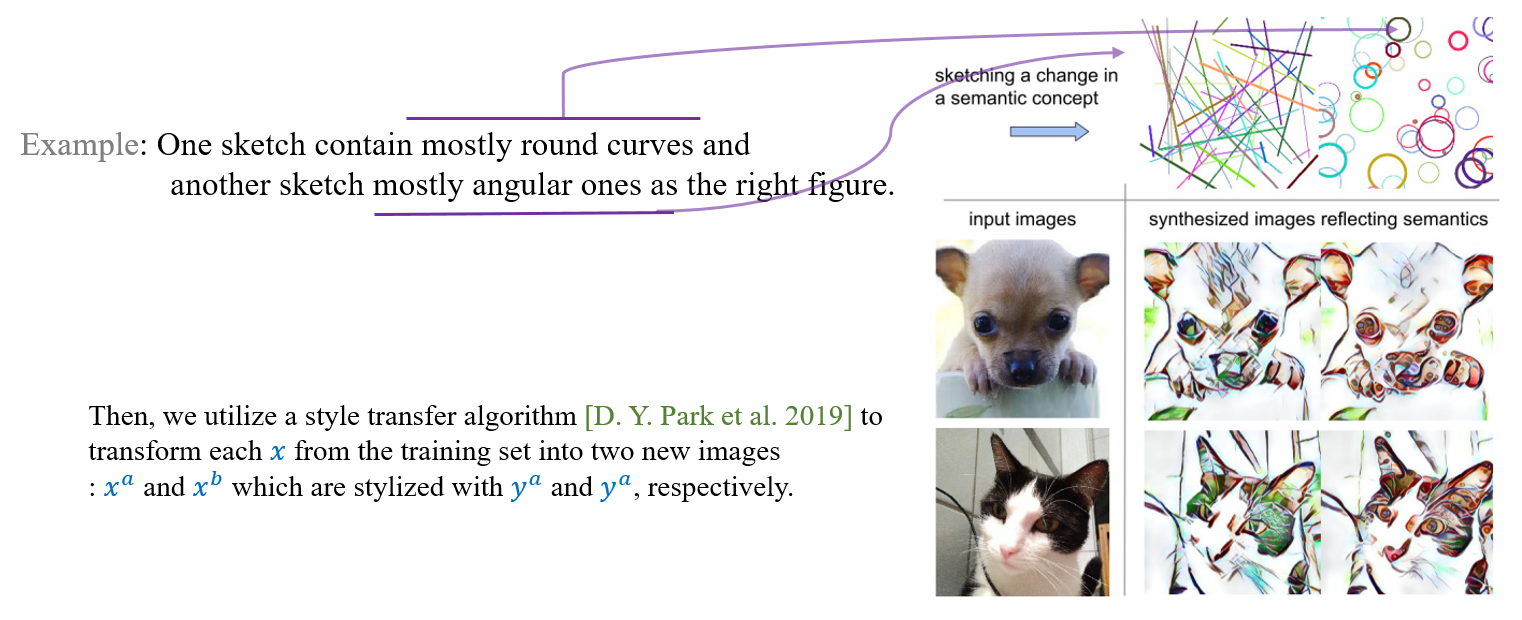
*Problem: * Most often, a sufficiently large number of image pairs is not easy to obtain.
*Solution: * A user only has to provide two sketches, \(y^a\) and \(y^b\) which demonstrate a change in concept.

2.3 Unsupervised Interpretations
Even without examples for changes in semantic factors, our approach can still produce disentangled factors, In this case, we minimized the negative log-likelihood of the marginal distribution of hidden representations \(z=E(x)\):
\[
L_{unsup}= - E_x \Vert T(E(x)) \Vert^2 - log \vert T'(E(x)) \vert. \quad \cdots Eq. (11)
\]

Reference
Esser, Patrick, Robin Rombach, and Bjorn Ommer. "A disentangling invertible interpretation network for explaining latent representations." Proceedings of the IEEE/CVF Conference on Computer Vision and Pattern Recognition. 2020.
'AI paper review > Explainable AI' 카테고리의 다른 글
| Counterfactual Explanation Based on Gradual Construction for Deep Networks (0) | 2022.03.10 |
|---|---|
| Interpretable And Fine-grained Visual Explanations For Convolutional Neural Networks (0) | 2022.03.09 |
| Interpretable Explanations of Black Boxes by Meaningful Perturbation (0) | 2022.03.07 |
| GradCAM (0) | 2022.03.07 |
