1. Counterfactual Explanation
Counterfactual Explanation: Given input data that are classified as a class from a deep network, it is to perturb the subset of features in the input data such that the model is forced to predict the perturbed data as a target class.
The Framework for counterfactual explanation is described in Fig 1.

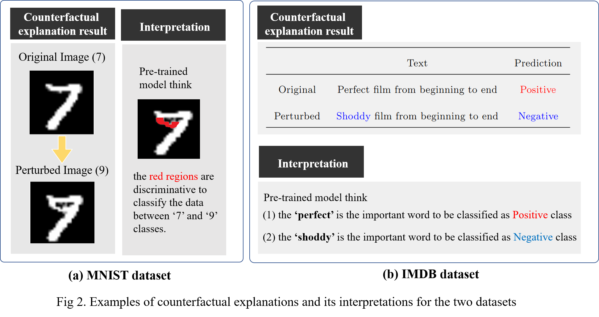
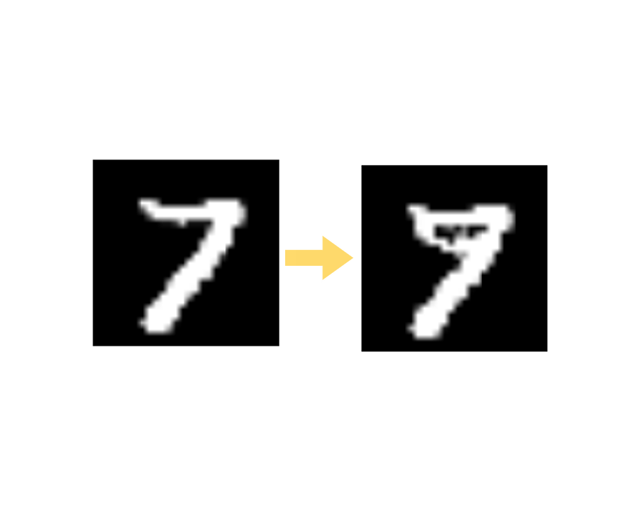
From perturbed data, we can interpret that the pre-trained model thinks the perturbed parts(regions) as the discriminative features between the original and target classes, such as Fig 2.

For this, the perturbed data for counterfactual explanation should satisfy two desirable properties.
- Explainability
- A generated explanation should be naturally understood by humans.
- Minimality
- Only a few features should be perturbed.
2. Method
To generate counterfactual explanations, we propose a counterfactual explanation method based on gradual construction that considers the statistics learned from training data. We particularly generate counterfactual explanations by iterating over masking and composition steps.

2.1 Problem definition
- Input (original) data: \(X \in \mathbb{R}^d \)
- Its predicted class : \(c_0\) under a pre-trained model \(f\)
- Perturbed data \(X'=(1-M) \circ X + M \circ C\)
- Binary mask: \(M = \{ 0,1 \}^d\)
- Composite: \(C\)
- Target class: \(c_t\)
- Desired classification score for the target class: \(\tau\)
The mask \(M\) indicates wheter to replace subset features of \(X\) with the composite \(C\) or to preserve the features of \(X\). The \(C\) represents newly generated feature values that will be replaced into a perturbed data \(X'\).
To produce perturbed data \(X'\) whose prediction will be a target class \(c_t\), we progressively search for an optimal mask and a composite. To this end, our method builds gradual construction that iterates over the masking and composition steps until the desired classification score \(\tau\) is obtained.
2.2 Masking step
The goal of the masking step is to select the most influential feature to
produce a target class from a pre-trained network as follows:
\[
i^\ast = argmax_i f_{c_t} (X+\delta e_i), \quad \cdots Eq. (1)
\]
where \(e_i\) is a one-hot vector whose value is 1 only for the \(i\)-th element, \(\delta\) is a non-zero real value and \(f_{c_t} \) is the classification score for the target class \(c_t\).
Suppose \(\delta = \bar{\delta} h \) where \(h\) is a non-zero and infinitesimal value and \(\bar{\delta}\) is a proper scalr to match the equality. Then, the Eq. (2) is approximated as the directional derivative with respect to \(X\).
\[
\begin{array}{l} f_{c_t} (X+\delta e_i) = f_{c_t} (X+\delta e_i) - f_{c_t} (X)+f_{c_t} (X) \cr \quad \quad \quad \quad \quad \; \,= f_{c_t} (X+ \bar{\delta} h e_i) - f_{c_t} (X)+f_{c_t} (X) \cr \quad \quad \quad \quad \quad \; \,= \frac{ f_{c_t} (X+ \bar{\delta} h e_i) - f_{c_t} (X) }{h}h+ f_{c_t} (X) \cr \quad \quad \quad \quad \quad \; \, \approx \bigtriangledown f_{c_t} (X) \bar{\delta} e_i h + f_{c_t} (X) \cr \quad \quad \quad \quad \quad \; \, = \bigtriangledown f_{c_t} (X) \delta e_i + R. \end{array} \quad \cdots Eq .(2)
\]
Since the \(\delta\) is a real value, we separately consider positive and negative cases in order to find an optimal \(i^\ast\).
\[
i^\ast= \left\{ \begin{array}{ll} max( \bigtriangledown f_t (X))_{i}, & if ; \delta >0, \cr
min( \bigtriangledown f_t (X))_i, & otherwise.
\end{array} \quad \cdots Eq .(3) \right.
\]
The \(t\) means \(c_t\). The \(max(\cdot)_i\) function returns an index that has a maximum value in the input vector and \(min(\cdot)_i\) is similarly defined.
Thus, we choose a sub-optimal idndex as
\[
\hat{i}^\ast = max ( | \bigtriangledown f_{c_t} (X) | )_i. \quad \cdots Eq. (4)
\]
In summary, each masking step selects an index in the descending order by calculating Eq. (5) and changes the zero value of mask \(M\) into one.
2.3 Composite step
After selecting the input feature to be modified, the composition step optimizes the feature value to ensure that the deep network classifies the perturbed data \(X'\) as the target class \(c_t\). To achieve this, the conventional approaches have proposed an objective function to improve the output score of \(c_t\) as follow:
\[
argmax_\epsilon f_{ c_t } (X+\epsilon) +R_\epsilon , \quad \cdots Eq. (5)
\]
where \( \epsilon= \{ \epsilon_1, \cdots , \epsilon_d \} \) is a perturbation variable and \(R_\epsilon \) is a regularization term.
However, this objective function causes an adversarial attack such as Failure images in Fig. 3. Then, we compared the contributions of logit scores (before the softmax layer) for each failure case and the training images that are classified as \(c_t\) from a pre-trained network. And, we discovered that there exists a notable difference between the two distributions as depicted in Fig 3.

Thus, we regard failure cases as the result of an n inappropriate objective function that maps the perturbed data onto a different logit space from the training data. To solve this problem, we instead force the logit space of \(X'\) to belong to the space of training data as follows:
\[
argmax_\epsilon f_{ c_t } (X+\epsilon) +R_\epsilon , \quad \cdots Eq. (6)
\]
where \(K\) is the number of classes, \(f'_k\) represents a logit score for a class \(k\), \(X_{i, c_t }\) denotes \(i\)-th training data that is classified into a target classes \(c_t\). \(N\) denotes the number of randomly sampled training data. In addition, we add a regularizer \(\lambda\) to encourage the values of \(X'\) to close to the input data \(X\).
As a result, Eq. (6) makes the composite \(C\) to improve the probability of \(c_t\) and also pushes the perturbed data towards belonging to the logit score distribution of a training data.
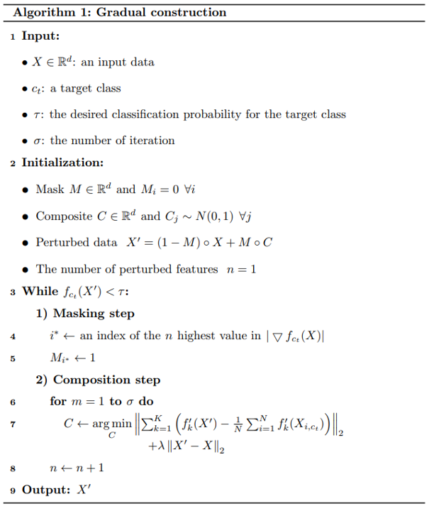
Overall, gradual construction iterates over the masking and composition steps until the classification probability of a target class is reached to a hyperparameter \(\tau\).
We present a pseudo-code in Algorithm 1.

3. Experiment


Reference
Kang, Sin-Han, et al. "Counterfactual Explanation Based on Gradual Construction for Deep Networks." arXiv preprint arXiv:2008.01897 (2020).
Github Code: Counterfactual Explanation Based on Gradual Construction for Deep Networks
'AI paper review > Explainable AI' 카테고리의 다른 글
| A Disentangling Invertible Interpretation Network for Explaining Latent Representations (0) | 2022.03.10 |
|---|---|
| Interpretable And Fine-grained Visual Explanations For Convolutional Neural Networks (0) | 2022.03.09 |
| Interpretable Explanations of Black Boxes by Meaningful Perturbation (0) | 2022.03.07 |
| GradCAM (0) | 2022.03.07 |
