1. How to explain the decision of black-box model??

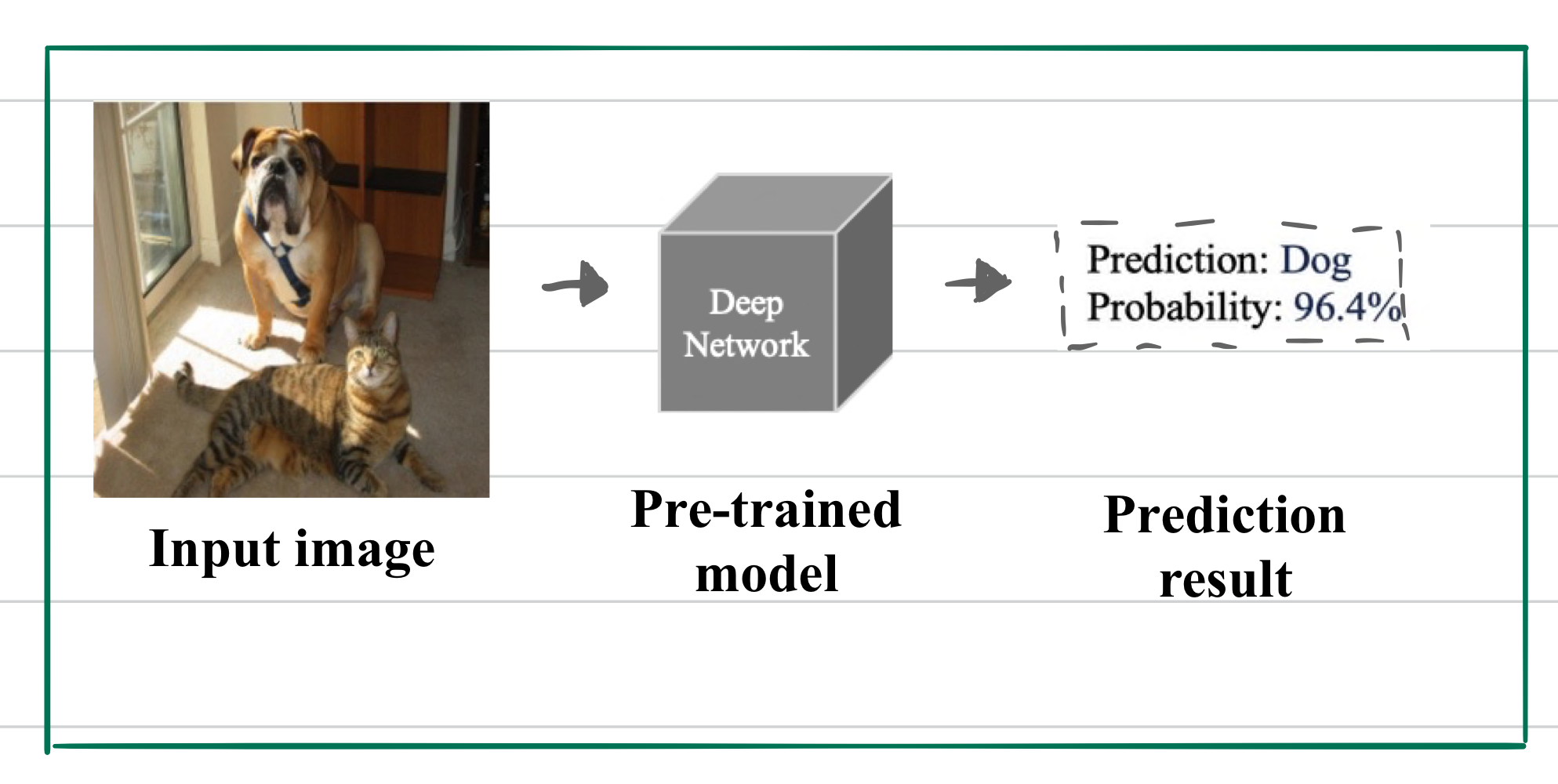
Given the left figure, we wonder that why the deep network predicts the image as "dog".
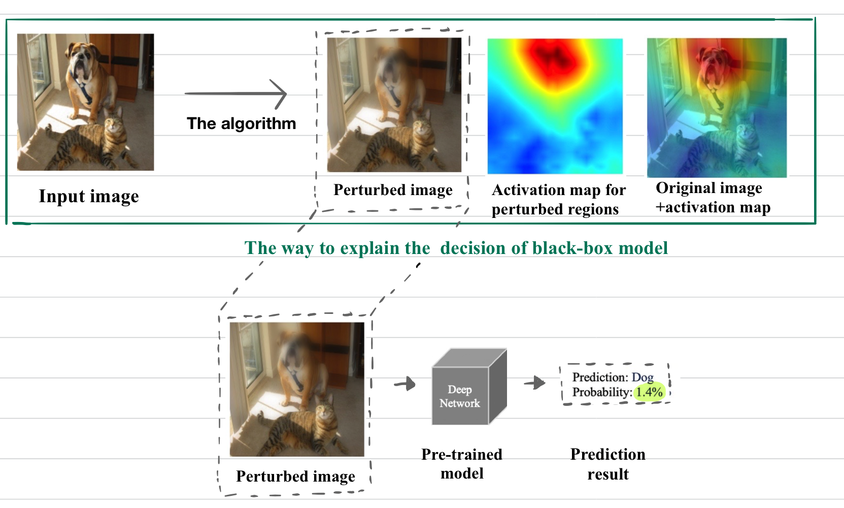
To gratify this curiosity, we aim to find the important regions of an input image to classify it as "dog" class.
\[ \downarrow \text{The idea} \]
If we find and remove THE REGIONS, the probability of the prediction significantly gets lower.
Note: removing the region represents that the regions are replaced with reference data (e.g. blurred, noise).

2. How to find the important regions to be classified as a target class?
2.1 Problem definition
- Input image: \(x_0 \)
- Black-box model: \(f \)
- Target class: \(c\)
- Prediction score for the target class: \( f_c(x_0)\)
2.2 Methods
In Interpretable Explanations of Black Boxes by Meaningful Perturbation, the goal is to find deletion (perturbation) regions that are maximally informative to the decision.
Let \( m:\lambda \rightarrow [0,1] \) be a mask, associating each pixel \( u \in \lambda \) with a scalar value \(m(u)\).
Then, the perturbation operator is defined as follows:
\[
\Phi(x_0: m)(u)= \left\{ \begin{array}{ll} m(u)x_0(u)+(1-m(u))u_0, & \text{constant}, \cr
m(u)x_0(u)+(1-m(u))\eta(u), & \text{noise}, \cr
\int g_{\sigma_0 m(u)} (v-u)x_0(v)dv, & \text{blur}
\end{array} \right.
\]
,where \(u_0\) is an average color, \(\eta(u)\) are i.i.d Gaussian noise samples for each pixel and \(\sigma_0\) is the maximum isotropic standard deviation of the Gaussian blur kernel \(g_\sigma\).
| If \(m(u)=1 \quad \) \(\rightarrow\) Preserve the original pixel |
| Elif \(m(u)=0 \quad \) \(\rightarrow\) Replace the original pixel with a pixel of reference data|
Note: I will define constant, noise, and blur as reference data \(R\).
2.2.1 The objective function
Find the smallest deletion mask \(m\) that causes the score \(f_c(\Phi (x_0:m)) \ll f_c(x_0)\) to drop significantly, where \(c\) is the target class. This represents that masked regions (pixels) were important to classify \(x_0\) as \(c\).
\[ m^*= argmin_{m \in [0,1]^\Lambda} \lambda \Vert 1-m\Vert_1+ f_c(\Phi(x_0:m))\]
,where \(\lambda\) encourages most of the mask to be turned off.
2.2.2 Dealing with artifacts
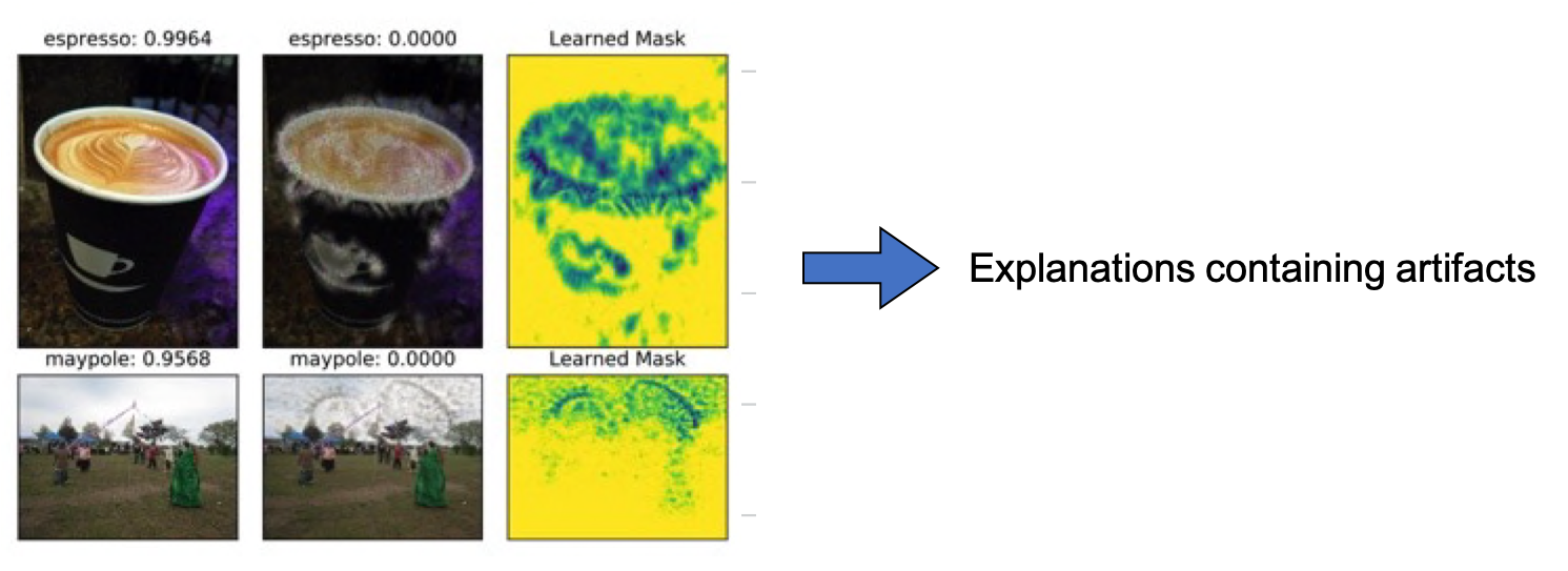
By committing to finding a single representative perturbation, our approach incurs the risk of triggering artifacts of the black-box model, like below figures.

To solve this problem, we suggest two approaches in generating explanations.
First, generalization for the mask
This means not relying on the details of a singly-learned mask \(m\). Hence, we reformulate the problem to apply the mask \(m\) stochastically, up to small random jitter.
Second, Total Variation (TV) regularization and upsampling
By using TV regularization and upsampling mask, we can encourage the result to have a simple, regular structure that can not be co-adapted to artifacts.
With these two modifications, the final objective function is follows:
\[min_{m \in [0,1]^\Lambda} \lambda_1 \Vert 1-m \Vert_1 + \lambda_2 \sum_u \Vert \bigtriangledown m(u) \Vert^\beta_\beta + \mathbb{E}_\tau [ f_c(\Phi (x( \cdot -\tau), m)) ] \]
,where second term represents TV regularization and third term indicates Generalization for the mask.
3. Implement details

3.1 Procedure of the upsampling method in the method

Reference
Fong, Ruth C., and Andrea Vedaldi. "Interpretable explanations of black boxes by meaningful perturbation." Proceedings of the IEEE International Conference on Computer Vision. 2017.
Github Code: Interpretable Explanations of Black Boxes by Meaningful Perturbation
'AI paper review > Explainable AI' 카테고리의 다른 글
| Counterfactual Explanation Based on Gradual Construction for Deep Networks (0) | 2022.03.10 |
|---|---|
| A Disentangling Invertible Interpretation Network for Explaining Latent Representations (0) | 2022.03.10 |
| Interpretable And Fine-grained Visual Explanations For Convolutional Neural Networks (0) | 2022.03.09 |
| GradCAM (0) | 2022.03.07 |
