
1. Goal
In Interpretable And Fine-grained Visual Explanations For Convolutional Neural Networks, authors propose an optimization-based visual explanation method, which highlights the evidence in the input images for a specific prediction.
1.1 Sub-goal
[A]: Defending against adversarial evidence (i.e. faulty evidence due to artifacts).
[B]: Providing explanations which are both fine-grained and preserve the characteristics of images, such as edges and colors.

2. Method
The authors provide local explanations, which focus on individual input. Given one data point, our method highlights the evidence on which a model bases its decision.
2.1 Perturbation based visual explanations
Perturbation based explanations can be defined as:
- Explanation by preservation: The smallest region of the image must be retained to preserve the original model output.
- Explanation by deletion: The smallest region of the image must be deleted to change the model output.
2.1.1 Problem definition
- CNN: \(f_{cnn}\)
- Input image: \( x \in \mathbb{R}^{3 \times H \times W}\)
- Output: \(y_x=f_{cnn} (x; \theta_{ cnn} ) \)
- Softmax scores: \(y^c_x\) of the different classes \(c\)
- Explanations: \(e^x_{c_T}\) for a target class \(c_T\)
2.1.2 The objective function
An explanation is computed by removing either relevant or irrelevant information from the image \(x\).
To do this, they use a mask based operator \(\Phi\), which computes a weighted average between the image \(x\) and a reference image \(r\), using a mask \(m_{c_T} \in [ 0,1 ]^{3 \times H \times W}\):

Authors introduce a similarity metric \(\varphi (y^{c_T}_x, y^{c_T}_e)\).
- Measuring the consistency of the model output generated by the explanation \(y^{c_T}_e\) and the output of the image \(y^{c_T}_x\) with respect to a target class \(c_T\)
- Typical choices for the metric (i) cross-entropy and (ii) negative softmax score of the target class
|If the explanation preserves the output of \(c_T\) \(\rightarrow\) the similarity is small |
|Elif the explanation manages to significantly drop the probability of \(c_T\) \(\rightarrow\) the similarity is large |
From the similarity metric, Let's define two versions of the objective functions.
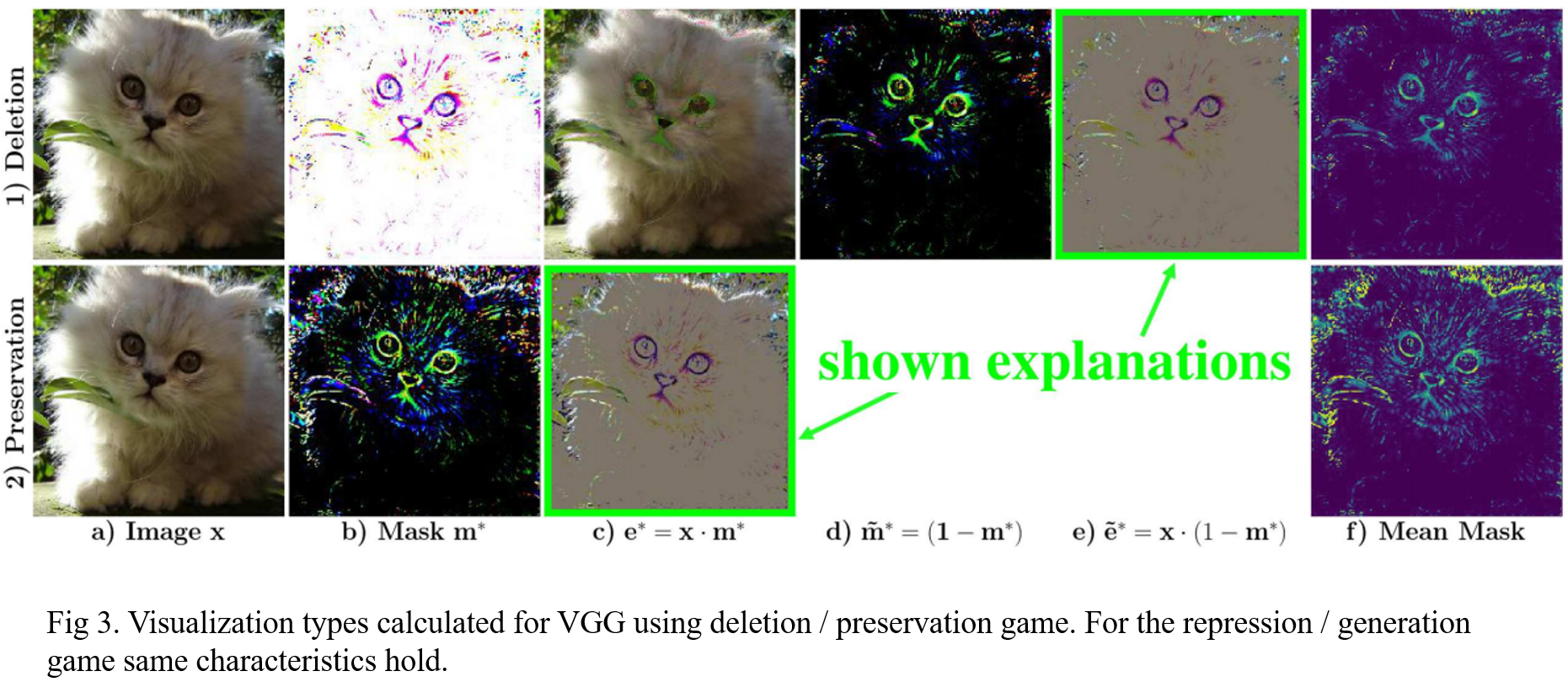
(1) Preserving game
Using the mask based definition of an explanation with a reference (\(r=0) \) as well as similarity metric, a preserving explanation can be computed by:
\[
\begin{array}{l} e^\ast_{ c_T } = m^\ast_{ c_T } \cdot x, \cr m^\ast_{ c_T }= argmin_{ m_{ c_T } } \varphi( y^{c_T}_x, y^{c_T}_e ) +\lambda \cdot R_m . \end{array} \quad \cdots Eq .(2)
\]
where \(R_m=\Vert m_{c_T} \Vert\) and \(\lambda\) encourages the mask to be sparse (i.e. many pixels are zero / appear black).
(2) Deletion game
We can compute a deleting explanation using:
\[
\begin{array}{l} e^\ast_{ c_T } = m^\ast_{ c_T } \cdot x, \cr m^\ast_{ c_T }= argmax_{ m_{ c_T } } \varphi( y^{c_T}_x, y^{c_T}_e ) +\lambda \cdot R_m . \end{array} \quad \cdots Eq .(3) \]
\(\lambda\) encourages masks Fig. 3 (b1) to contain mainly ones (i.e. appear white) and only small entries at pixels, which provide the most prominent evidence for the target class.
To solve the optimization in Eq. (2) and (3), we utilize Stochastic Gradient Descent (SGD and start with an explanation \(e^0_{c_T} =1 \cdot x\) identical to the original image (i.e. a mask initialized with ones).
2.2 Defending against Adversarial Evidence
CNNs have been proven susceptible to adversarial images. Due to the computational similarity of adversarial methods and optimization-based visual explanation approaches, adversarial noise is also a concern for our method.
To tackle this problem, the authors propose a novel adversarial defense that filters gradients during backpropagation in a targeted way. The basic idea is: A neuron within a CNN is only allowed to be activated by the explanation \(e_{c_T}\) if the same neuron was also activated by the original image (x).
If we regard neurons as indicators for the existence of features (e.g. edges, object parts, ...), the proposed constraint enforces that the explanation \(e_{c_T}\) can only contain features that exist at the same location in the original image (x) as follow:
\[
\left\{ \begin{array}{ll} 0 \leq h^l_i (e_{c_T}) \leq h^l_i (x), & if \; h^l_i (x) \geq 0, \cr 0 \geq h^l_i (e_{c_T}) \geq h^l_i (x), & otherwise, \end{array} \right. \quad \cdots Eq. (4)
\]
where \(h^l_i\) is the activation of the \(i\)-th neuron in the \(l\)-th layer of the network after the nonlinearity. This constraint is applied after all nonlinearity-layers (e.g. ReLU-Layers) of the network, besides the final classification layer.
To solve the optimization with subject to Eq. (4), one could incorporate the constraints via a penalty function by adding an additional layer \( \overline{h}^l_i \) after each nonlinearity:
\[
\begin{array}{l} \overline{h}^l_i ( e_{c_T} ) = min (bu, max(bl, h^l_i (e_{ c_T }))), \cr bu =max(0,h^l_i (x)), \cr bl= min (0, h^l_i (x)), \end{array} \quad \cdots Eq. (5)
\]
where \(h^l_i(e_{c_T})\) is the acutal activation of the origianl nonlinearity-layer and \( \overline{h}^l_i (e_{c_T})\) the adjusted activation after ensuring the bounds \(bu\), \(bl\) of the original input.
However, since this method changes the architecture of the model which we explain, do clip gradients in the backward pass of the optimization, which leads to a violation of Eq. (4). This is equivalent to adding an additional clipping-layer after each nonlinearity which acts as the identity in the forward pass and uses the gradient update of Eq. (5) in the backward pass. When backpropagating an error-signal \(\overline{\gamma}_i^l\) through the clipping-layer, the gradient update rule for the resulting error \(\gamma_i^l\) is defined by:
\[
\gamma^l_i=\overline{\gamma}^l_i \cdot [ h^l_i (e_\{ c_T \} ) \leq bu ] \cdot [ h^l_i ( e_{c_T }) \geq bl ] , \quad \cdots Eq. (6)
\]
where \([ \cdot ]\) is the indicator function and \(bl\), \(bu\) the bounds computed in Eq. (5). This clipping only affects the gradients of the similarity metric \(\varphi ( \cdot , \cdot )\) which are propagated through the network. The result examples of our adversarial defense are shown in Fig 4.

Reference
Wagner, Jorg, et al. "Interpretable and fine-grained visual explanations for convolutional neural networks." Proceedings of the IEEE/CVF Conference on Computer Vision and Pattern Recognition. 2019.
'AI paper review > Explainable AI' 카테고리의 다른 글
| Counterfactual Explanation Based on Gradual Construction for Deep Networks (0) | 2022.03.10 |
|---|---|
| A Disentangling Invertible Interpretation Network for Explaining Latent Representations (0) | 2022.03.10 |
| Interpretable Explanations of Black Boxes by Meaningful Perturbation (0) | 2022.03.07 |
| GradCAM (0) | 2022.03.07 |