1. Introduction
Filter Decomposition (FD): Decomposing a weight tensor into multiple tensors to be multiplied in a consecutive manner and then getting a compressed model.
1.1 Motivation
Well-known low-rank approximation (i.e. FD) methods, such as Tucker or CP decomposition, result in degraded model accuracy because decomposed layers hinder training convergence.
1.2 Goal
To tackle this problem, they propose a new training technique, called DeepTwist, that finds a flat minimum in the view of low-rank approximation without a decomposed structure during training.
That is, they retain the original model structure without considering low-rank approximation. Moreover, because the method preserves the original model structure during training, 2-dimensional low-rank approximation demanding lowering (such as im2col) is available.
2. Training Algorithm for Low-Rank Approximation
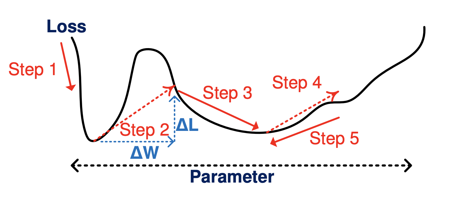
Note that FD methods incur the accuracy drop from the original network because of an approximation error given a rank. If so, in terms of loss surface, which position of parameters is appropriate before applying FD in the below figure?

As you already expect, the right position of parameters is less sensitive to accuracy drop (loss variance). That is, the underlying principle of the proposed training algorithm is to find a particular local minimum of flat loss surface, robust to parameter errors induced by low-rank approximation.
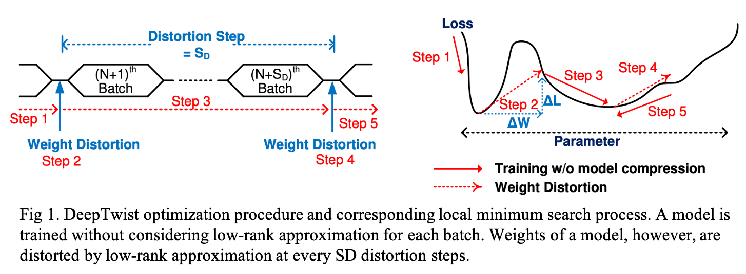
The proposed scheme preserves the original model structure and searches for a local minimum well suited for low-rank approximation. The training procedure for low-rank approximation, called DeepTwist, is illustrated in Fig. 1.
- Step by Step
- Training \( S_D \) batches.
- At each weight distortion step, parameters are decomposed into multiple tensors following low-rank approximation (e.g. CP, tucker).
- Those decomposed tensors are multiplied to reconstruct the original tensor form.
- If a particular local minimum is not flat enough, training procedure escapes such a local minimum through a weight distortion step (step 2).
- Otherwise, the optimization process is continued in the search space around a local minimum (steps 4 and 5).
2.1 Determining the best distortion step \(S_D\)
Determining the best distortion step \( S_D \) is important in training procedure. The loss function of a model \( L(w)\) is approximated as:
\[
L(w) \simeq L(w_0) + (w - w_0)^{\top} (H(w_0)/2) (w - w_0), \quad \cdots (1)
\]
using a local quadratic approximation (taylor series).
- Parameter set: \( w \)
- Set of parameters at a local minimum: \( w_0 \)
- Hessian of \( L \): \( H \)
- Learning rate: \( \gamma \)
Then, \( w \) can be updated by gradient descent as follows:
\[
w_{t+1} = w_t - \gamma \frac{\partial L}{\partial w} |_{ w = w_t } \simeq w_t - \gamma H(w_0)(w_t - w_0) \quad \cdots (2)
\]
Thus, after \( S_D \) steps, you obtain \( w_{ t+ S_D } = w_0 + (I - \gamma H(w_0))^{S_D} (w_t - w0)\), where \( I \) is identity matrix. Suppose that \( H \) is positive semi-definite and all elements of \( I - \gamma H(w_0) \) are less than 1.0, large \( S_D \) converges to \( w_0 \).
Correspondingly, large \( S_D \) is preferred for this proposed method. Large \( S_D \) is also desirable to avoid stochastic variance from the batch selection. However, Too large of a \( S_D \) yields fewer opportunities to escape local minima especially when the learning rate has decayed. In practice, \( S_D \) falls in the range of 100 to 5000 steps.
3. Tucker Decomposition Optimized by DeepTwist
First of all, Tucker decomposition is described as below:
\[
K'_{i, j, s, t} = \sum^{R_s} \sum^{R_t} C P^S P^T \quad \cdots (3)
\]
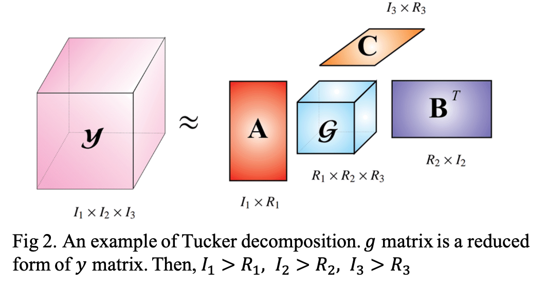
- Original 4D kernel tensor: \( K = \mathcal{R}^{ d \times d \times S \times T }\).
- Kernel dimension: \( d \times d \).
- Input feature map size: \( S \).
- Output feature map size: \( T \).
- Approximated 4D kernel tensor: \( K' = \mathcal{R}^{ d \times d \times S \times T }\).
- Reduce kernel tensor: \( C = C_{ i, j, r_s, r_t} \).
- The rank for input feature map dimension: \( R_s \).
- The rank for output feature map dimension: \( R_t \).
- 2D filter matrices to map \( C_{ i, j, r_s, r_t} \) to \( K_{ i, j, r_s, r_t } \): \( P^S, P^T \).
Each component is obtained to minimize the Frobenius norm of \( ( K_{ i, j, r_s, r_t } - K'_{ i, j, r_s, r_t} ) \). As a result, one convolution layer is divided into three convolution layers, specifically, (1×1) convolution for \( P^S \), (d × d) convolution for \( C_{ i, j, r_s, r_t } \), and (1 × 1) convolution for \( P^T \).
DeepTwist training algorithm is conducted for Tucker decomposition as follows:
- Perform normal training for \( S_D \) steps (batches) without considering Tucker decomposition.
- Calculate \( C \), (( P^s \) and \( P^T \) using Tucker decomposition to obtain \( K' \).
- Replace \( K \) with \( K' \) (a weight distortion step in Fig. 1).
- Go to Step 1 with updated \( K \).
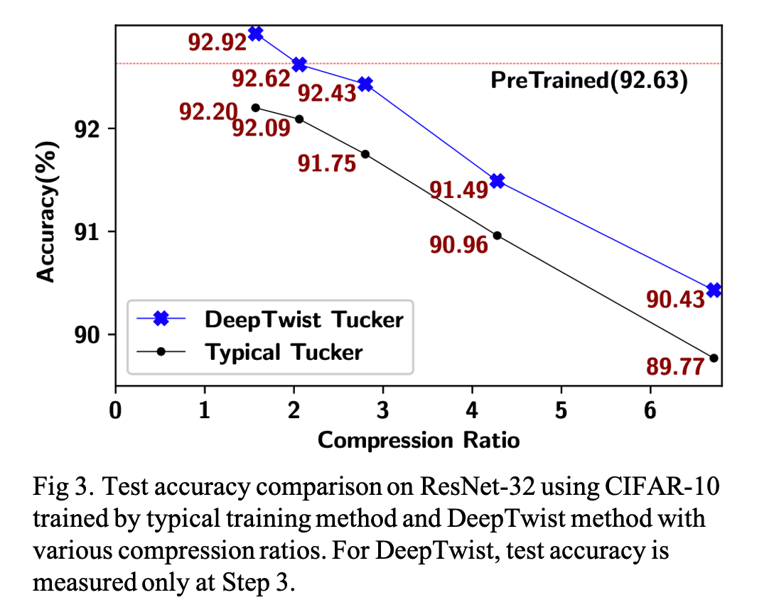
Using the pre-trained ResNet-32 model with CIFAR-10 dataset, compare two training methods for Tucker decomposition: 1) typical training with a decomposed model and 2) DeepTwist training (\( S_D \) = 200). The result is as follows.
4. 2-Dimensional SVD Enabled by DeepTwist
4.1 Issues of 2D SVD on Convolution Layers
Convolution can be performed by matrix multiplication if an input matrix is transformed into a Toeplitz matrix with redundancy and a weight kernel is reshaped into a T × (S × d × d) matrix (i.e., a lowered matrix). Then, commodity computing systems (such as CPUs and GPUs) can use libraries such as Basic Linear Algebra Subroutines (BLAS) without dedicated hardware resources for convolution.
For BLAS-based CNN inference, reshaping a 4D tensor \( K \) and performing SVD is preferred for low-rank approximation rather than relatively inefficient Tucker decomposition. However, because of lowering steps, two decomposed matrices by SVD do not present corresponding (decomposed) convolution layers. As a result, the fine-tuning requiring a structurally modified model for training is not allowed. But, DeepTwist does not alter the model structure during training.
4.2 Tiling-Based SVD for Skewed Weight Matrices
A reshaped kernel matrix \( K \in \mathcal{R}^{ T \times (S \times d \times d)\ } \) is usually a skewed matrix where row-wise dimension (\( n \)) is smaller than column-wise dimension (\( m \)) as shown in Fig. 4 (i.e., \( n \ll m \)). A range of available rank \( r \) for SVD, then, is constrained by small \( K \) and the compression ratio is approximated
to be \( n/r \). If such a skewed matrix is divided into four tiles as shown in Fig. 4 and the four tiles do not share many common characteristics, then tiling-based SVD can be a better approximator and rank \( r \) can be further reduced without increasing approximation error. Moreover, fast matrix multiplication is usually implemented by a tiling technique in hardware to improve the weight reuse rate.
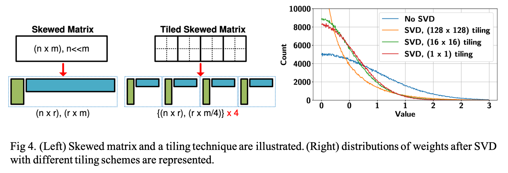
They tested a (1024 × 1024) random weight matrix in which elements follow a Gaussian distribution. A weight matrix is divided by (1×1), (16×16), or (128×128)tiles (then, each tile is a submatrix of (1024×1024), (64×64), or (8×8) size). Each tile is compressed by SVD to achieve the same overall compression ratio of 4× for all of the three cases. As described in Fig. 4. (on the right side), increasing the number of tiles tends to increase the count of near-zero and large weights.
They applied the tiling technique and SVD to the 9 largest convolution layers of ResNet-32 using the CIFAR-10 dataset. Weights of selected layers are reshaped into 64 × (64 × 3 × 3) matrices with the tiling configurations described in Table 1. DeepTwist performs training with the same learning schedule and SD(=200) used in Section 3.

Reference
Lee, Dongsoo, et al. "Learning low-rank approximation for cnns." arXiv preprint arXiv:1905.10145 (2019).
'AI paper review > Model Compression' 카테고리의 다른 글
| Learning Features with Parameter-free Layers 논문 리뷰 (0) | 2022.04.28 |
|---|---|
| Few Sample Knowledge Distillation for Efficient Network Compression (0) | 2022.03.11 |
| Knowledge Distillation via Softmax Regression Representation Learning (0) | 2022.03.10 |
| EagleEye: Fast Sub-net Evaluation for Efficient Neural Network Pruning (0) | 2022.03.10 |
| Data-Free Knowledge Amalgamation via Group-Stack Dual-GAN (0) | 2022.03.09 |
