EagleEye: Fast Sub-net Evaluation for Efficient Neural Network Pruning

1. Introduction

Pruning: Eliminating the computational redundant part of a trained DNN and then getting a smaller and more efficient pruned DNN.

1.1 Motivation

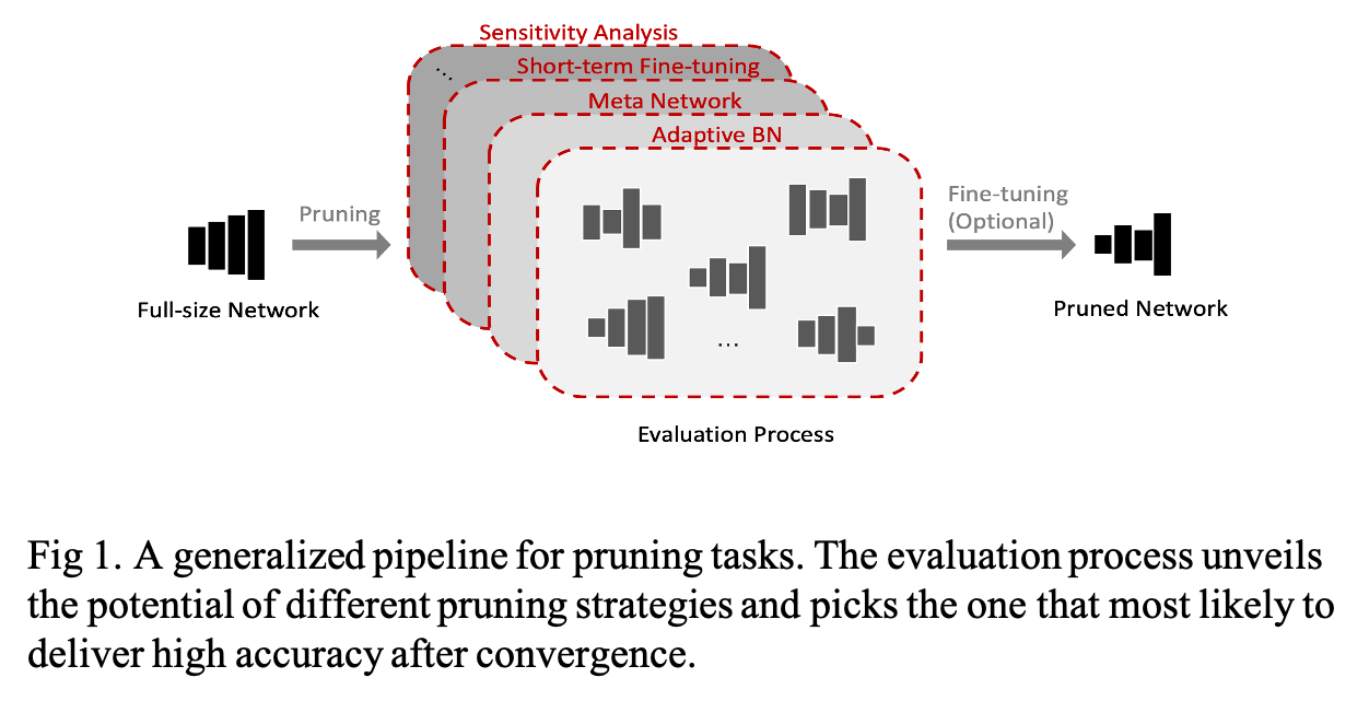
The important thing to prune a trained DNN is to obtain the sub-net with the highest accuracy with reasonably small searching efforts. Existing methods to solve this problem mainly focus on an evaluation process. The evaluation process aims to unveil the potential of sub-nets so that the best pruning candidate can be selected to deliver the final pruning strategy such as Fig 1.

 

However, the existing methods for the evaluation process are either (i) inaccurate or (ii) complicated.

 

For (i), the winner sub-nets from the evaluation process do not deliver high accuracy.
For (ii), the evaluation process relies on computationally intensive components or is highly sensitive to some hyperparameters.

1.2 Goal

To solve these problems, the authors propose a pruning algorithm called EagleEye that is a faster and more accurate evaluation process. The EagleEye adopt the technique of adaptive batch normalization.

2. Method

 

A typical pruning pipeline is shown in Fig 2. In this pipeline, the authors aim to structure filter pruning approaches:

$$(r_1,..,r_L{)}^{\ast }=argmi{n}_{r_1,..,r_L}\mathcal{L}(\mathcal{A}(r_1,..,r_L;w)),s.t.\mathcal{C}<cs,\cdots Eq.(1)$$

where $\mathcal{L}$ is the loss function, $cs$ is a constraint and $\mathcal{A}$ is the neural network model. $r_l$ is the pruning ratio applied to the $l-th$ layer. Given some constraints $\mathcal{C}$ (e.g. latency, total parameters), a combination of pruning ratios $(r_1,\cdots ,r_L)$ is applied. the authors consider pruning task as finding the optimal pruning strategy, denoted as $(r_1,\cdots ,r_L{)}^{\ast }$, that achieves the highest accuracy of the pruned model.

2.1 Motivation

The authors found that the existing evaluation processes, called vanilla evaluation, do not satisfy that the sub-nets with higher evaluation accuracy are expected to also deliver high accuracy after fine-tuning as shown in Fig 3. In Fig 3 (a). left, the red bars form the histogram of accuracy collected from doing a vanilla evaluation with the 50 pruned candidates. And the gray bars show the situation after fine-tuning these 50 pruned networks.

 

However, there is a huge difference in accuracy distribution between the two results. In addition, Fig 3 (b) indicates that it might not be the weights that mess up the accuracy at the evaluation stage as only a gentle shift in weight distribution is observed during fine-tuning for the 50 networks.

 

Interestingly, the authors found that it is the batch normalization layer that largely affects the evaluation. More specifically, the sub-networks use moving mean and moving variance of Batch Normalization (BN) inherited from the full-size model. The outdated statistical values of BN layers eventually drag down the evaluation accuracy and then break the correlation between evaluation accuracy and the final converged accuracy of the pruning candidates.

 

To quantitatively demonstrate the problem of vanilla evaluation, let's symbolize the original BN as follows:

$$y=\gamma \frac{x-\mu }{{\sigma }^2+ϵ}+\beta ,\cdots Eq.(2)$$

where $\beta$ and $\gamma$ are trainable scale and bias terms. $ϵ$ is a term with a small value to avoid zero division. For a mini-batch with size $N$, the statistical values of $\mu$ and ${\sigma }^2$ are calculated as below:

$${\mu }_B=E[x_B]=\frac{1}{N}\sum _i^N{x}_i,{\sigma }_B^2=Var[x_B]=\frac{1}{N-1}\sum _i^N(x_i-{\mu }_B{)}^2.\cdots Eq.(3)$$

During training, $\mu$ and ${\sigma }^2$ are calculated with the moving mean and variance:

$${\mu }_t=m{\mu }_z+(1-m){\mu }_B,{\sigma }_t^2=m{\sigma }_z^2+(1-m){\sigma }_B,\cdots Eq.(4)$$

where $z=t-1$, $m$ is the momentum coefficient and subscript $t$ refers to the number of training iterations. And if the total number of training iterations is $T$, ${\mu }_T$ and ${\sigma }_T^2$ are used in the testing phase.

These two items are called global BN statistics, where "global" refers to the full-size model.

2.2 Adaptive Batch Normalization

Because the global BN statistics are outdated to the sub-nets from vanilla evaluation, we should re-calculate ${\mu }_T$ and ${\sigma }_T^2$ with adaptive values by conducting a few iterations of inference on part of the training sets. Concretely, the authors freeze all the network parameters while resetting the moving average statistics. Then, do update the moving statistics by a few iterations of only forward-propagation, using Eq. (4). The authors denote adaptive BN statistics as ${\hat{\mu }}_T$ and ${\hat{\sigma }}_T^2$.

 

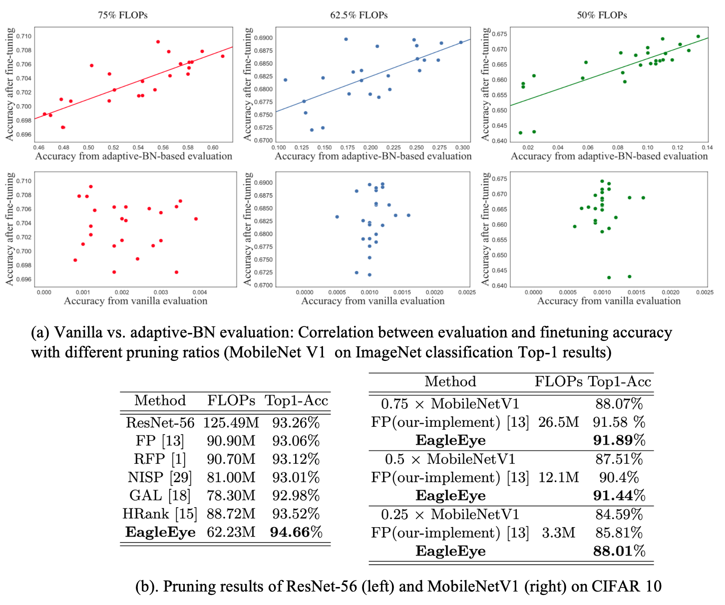
To validate the effectiveness of the proposed method, Fig 4. shows that adaptive BN delivers evaluation accuracy with a stronger correlation, compared to the vanilla evaluation. The correlation measurement is conducted by Pearson Correlation Coefficient (PCC).

As another piece of evidence, the authors compare the distance of BN statistical values between true statistics. They consider the true statistics as ${\mu }_{val}$, ${\sigma }_{val}$ sampled from validation data. As you expect, the adaptive BN provides closer statistical values to the true values while global BN is way further as shown in Fig 5. (each pixel in the heatmaps represents a distance.)

2.3 EagleEye pruning algorithm

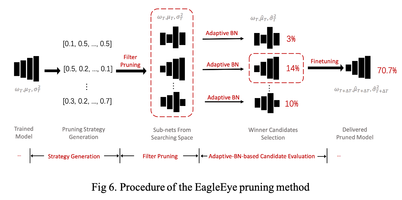
The overall procedure of EagleEye is described in Fig 6. The procedure contains three parts, (1) pruning strategy generation, (2) filter pruning, and (3) adaptive BN-based evaluation.

1. Strategy generation
Generation randomly samples $L$ real numbers from a given range $[0,R]$ to form a pruning strategy $(r_1,\cdots ,r_L{)}^{\ast }$. $R$ is the largest pruning ratio applied to a layer. This is a Monte Carlo sampling process with a uniform distribution for all layer-wise pruning rates.

 

2. Filter pruning process
Similar to a normal filter pruning method, the filters are firstly ranked according to their $L1$-norm and the $r_l$ of the least important filters are trimmed off.

 

3. The adaptive-BN based candidate evaluation module
Given a pruned network, it freezes all learnable parameters and traverses through a small amount of data in the training set to calculate the adaptive BN statistics. In practice, the authors sampled 1/30 of the total training set for 100 iterations in ImageNet dataset. Next, the module evaluates the performance of the candidate networks on a small part of training set data, called sub-validation set, and picks the top ones in the accuracy ranking as a winner candidate.

 

4. Fine-tuning
The fine-tuning will be applied to the winner candidate network.

3. Experiments

 

Reference

Li, Bailin, et al. "Eagleeye: Fast sub-net evaluation for efficient neural network pruning." European Conference on Computer Vision. Springer, Cham, 2020.

 

 

Github Code: Eagleeye