1. Goal
The goal is to perform Data-free Knowledge distillation.
Knowledge distillation: Dealing with the problem of training a smaller model (Student) from a high capacity source model (Teacher) so as to retain most of its performance.
As the word itself, We perform knowledge distillation when there is no original dataset on which the Teacher network has been trained. It is because, in real world, most datasets are proprietary and not shared publicly due to privacy or confidentiality concerns.
To tackle this problem, it is necessary to reconstruct a dataset for training Student network. Thus, in this paper, the authors propose a data-free knowledge amalgamate strategy to craft a well-behaved multi-task student network from multiple single/multi-task teachers.
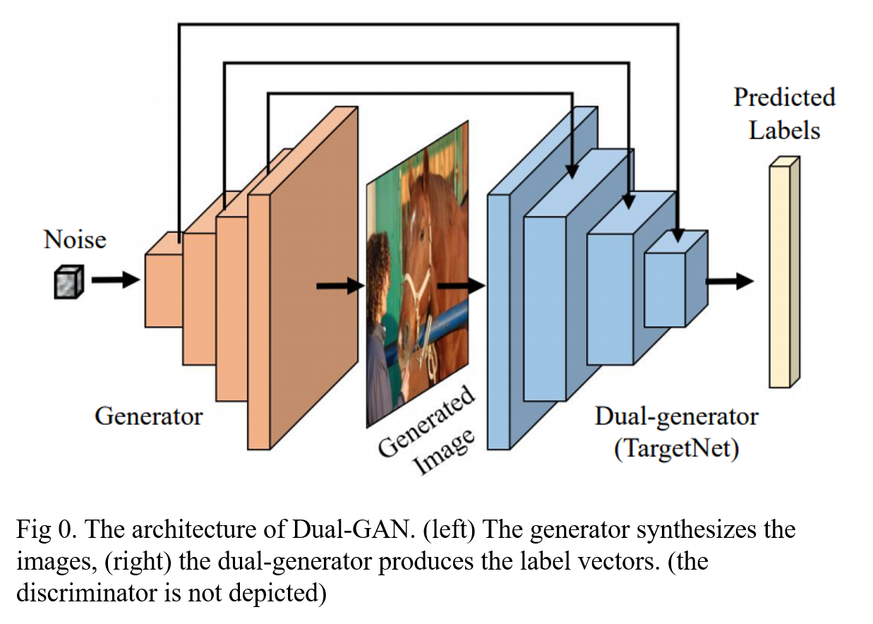
For this, the main idea is to construct the group-stack generative adversarial networks (GANs) which have two dual generators. First, one generator is trained to collect the knowledge by reconstructing the images approximating the original dataset. Then, a dual generator is trained by taking the output from the former generator as input. Finally, we treat the dual part generator as the TargetNet (Student network) and regroup it.
The architecture of Dual-GAN is shown in Fig 0.
2. Problem Definiton
In Data-Free Knowledge Amalgamation via Group-Stack Dual-GAN, The authors aim to explore a more effective approach to train the student network (TargetNet), only utilizing the knowledge amalgamated from the pre-trained teachers. The TargetNet is designed to deal with multiple tasks and learns a customized multi-branch network that can recognize all labels selected from separate teachers.
- The number of the customized categories: \( C \)
- Label vector: \( Y_{cst}= \{ y_1, \cdots , y_C \} \subseteq \{ 0 , 1 \}^C \)
- TargetNet: \( \mathcal{T} \)
- Handling multiple tasks on the \( Y_{cst} \)
- Pre-trained teachers: \( \mathcal{A} = \{ \mathcal{A}_1, \cdots, \mathcal{A}_M \} \)
- For each teacher \( m \) , a \( T_m\) -label classification task :\( Y_m= \{ y^1_m, \cdots , y^{T_m}_m \} \)
- Feature maps in the \(b\)-th block of the \(m\)-th pre-trained teacher: \( F^b_m \)
The teacher networks are in the constraint: \( Y_{cst} \subseteq \bigcup^M_{ m=1 } Y_m \), which reveals that either the full or the subset of classification labels is an alternative for making up the customized task set.
3. Method
The process of obtaining the well-behaved TargetNet with the proposed data-free framework contains three steps.
- The generator \( G(z): z \rightarrow \mathcal{I} \) is trained with knowledge amalgamation in the adversarial way, where the images in the same distribution of the original dataset can be manufactured. Note that \(z\) is the random noise and \( \mathcal{I} \) denotes the image.
- The dual generator \( \mathcal{T} (\mathcal{I}): \mathcal{I} \rightarrow Y_{cst} \) is trained with generated samples from \( G \) in the block-wise way to produce multiple predict labels. Note that \( Y_{cst} \) is the predicted labels.
- After training the whole dual-GAN, The dual-generator is modified as TargetNet for classifying the customized label set \( Y_{cst} \)
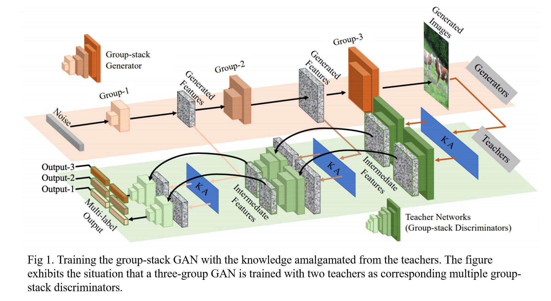
The overall training procedure of group-stack GAN is depicted in Fig 1.
3.1 Amalgamating GAN
First, introduce the arbitrary vanilla GAN. The GAN performs a minmax game between a generator \(G(z): z \rightarrow \mathcal{I} \) and a discriminator \( D (x) : \mathcal{I} \rightarrow [0,1] \), and the objective function can be defined as:
\[
L_{GAN}= \mathbb{E}_x [ log \mathcal{D} ( \mathcal{I})] +\mathbb{E} [log(1-D(G(z)))]. \quad \cdots Eq. (1)
\]
However, since the absence of real data, we can not perform training by Eq. (1). Then, several modification have been made as follows.
3.1.1 Group-stack GAN
The first modification is the group-stack architecture. The generator is designed to generate not only synthesized images but also the intermediated activations aligned with the teachers.
Thus, we set \( B \) as the total group number of generators, which is the same as the block numbers of the teacher and the student networks. In this way, the generator can be denoted as a stack of \(B\) groups \( \{G^1, \cdots, G^B \} \), from which both the image \( \mathcal{I}_g \) and the consequent activation \( F^j_g \) at group \( j \) are synthesized from a random noise \( z \):
\[
\begin{array}{l} F^1_g=G^1(z) \cr F^j_g=G^j(F^\{ j-1 \}_g) \; 1 < j \leq B, \end{array} \quad \cdots Eq .(2)
\]
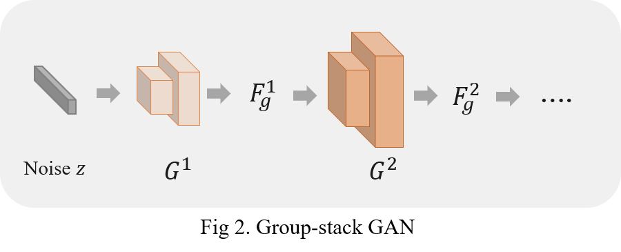
when \( j=B \), the output of the \( B\)-th group \(G^B\) is \( F^B_g\), which is also thought as the final generated image \( \mathcal{I}_g \).
Since both the architecture of generator \(G^j\) and discriminator \(D^j\) are symmetrical, the group adversarial pair is presented as \( [ \{ G^1,D^1\}, \cdots ,\{ G^B,D^B\} ] \). In this way, the satisfying \(G^{j \ast}\) can be acquired by:
\[
G^{j \ast }=argmin_\{ G^j \} \mathbb{E}_z [log(1-D^{j*} (G^j (F^{j-1}_g)))] \quad \cdots Eq. (3)
\]
where \( 1 \leq j \leq B \) and \( D^{j*} \) is the optimal \(j\)-group discriminator. We transfer the discriminator to designing a plausible loss function to calculate the difference between the generated samples and the real ones. Thus, we take the teacher network \( \mathcal{A} \) to constitute each \(D^j\):
\[
D^j \leftarrow \bigcup^j_{i=1} \{ \mathcal{A}^{B-j+i} \} \quad \cdots Eq. (4)
\]
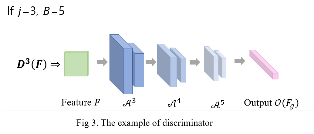
During the training for the group pair \( \{ G^j, D^j \} \), only \(G^j \) is optimized with discriminator \(D^j \) is fixed, whose output is for classifying multiple labels. We make use of several losses to constraint the output of \(D^j \) to motivate the real data's response.
The output for \( D\) is \(\mathcal{O} ( F_g) = \{ y^1, \cdots , y^C \} \), with the predict label as \(t^i \):
\[
t^i= \left\{ \begin{array}{ll} 1 & y^i \geq \epsilon, \cr 0 & y^i < \epsilon, \end{array} \right. \quad \cdots Eq. (5)
\]
where \( 1 \leq i \leq C \) and \( \epsilon \) is set to be 0.5 in the experiment. Then the one-hot loss function can be defined as:
\[
L_{oh}= \frac{1}{C}\sum_i l(y^i, t^i), \quad \cdots Eq. (6)
\]
where \( l \) is the cross-entropy and \( L_{oh} \) enforces the outputs of the generated samples to be close to one-hot vectors.
In addition, the outputs need to be sparse, since an image in the real world can't be tagged with dense labels which are the descriptions for different situations. So, an extra discrete loss function is proposed:
\[
L_{dis}= \frac{1}{C} \sum_i \vert y^i \vert, \quad \cdots Eq. (7)
\]
which is known as L1-norm loss function. Finally, combining all the losses, the final objective function can be obtained:
\[
L_{gan}= L_{oh} + \alpha L_a + \beta L_{ie} + \gamma L_{dis }, \quad \cdots Eq. (8)
\]
where \( \alpha, \beta \) and \( \gamma \) are the hyperparameters for balancing different loss items. \( L_a \) and \( L_{ie} \) are the activation loss and information entropy loss functions and described in the paper "Data-Free Learning of Student Networks"[H. Chen et al., 2019].
3.1.2 Multiple Targets
Since the TargetNet is customized to perform multi-label classifications learning from multiple teachers, the generator should generate samples containing multiple targets. As a result, for the \(j \)-th group generator \( G^j \), authors construct multiple group-stack discriminators \( \{ D^j_1, \cdots, D^j_M \} \) in concert with teachers specializing in different task sets by Eq. (4).
In order to amalgamate multi-knowledge into the generator by \( \{ D^j_m \}^M_{m=1} \), the teacher-level filtering is applied to \(F^j_g \). And this filtering is conducted as:
\[
F^{f,m}_g=f^j_m (F^j_g), \quad \cdots Eq. (9)
\]
where the filtering function \( f^j_m \) is realized by a light learnable module consisting of a global pooling layer and two fully connected layers. \( F^{j,m}_g \) is the filtered generated features that approach the output feature distribution of \( \mathcal{A}^{B-j}_m \). The output of discriminator is donated as \( \mathcal{O}_m (F^j_g) = D^j_m (F^{j,m}_g \).
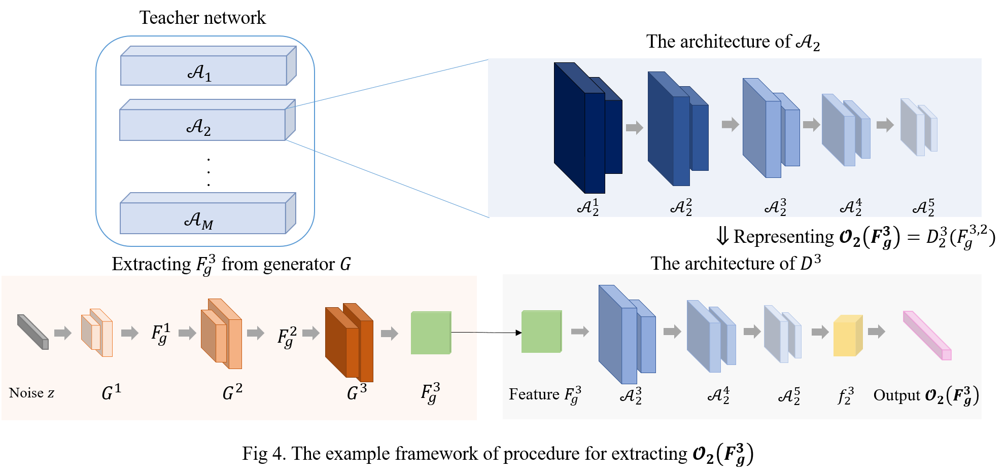
The for the generated features \( F^j_g \) from \( G^j \), we collect from the multi-discriminator the \( M \) prediction sets \( \{ \mathcal{O}_1(F^j_g), \cdots , \mathcal{O}_M (F^j_g) \} \), which are:
\[
\mathcal{O}_g (F^j_g) = \bigcup^M_m \mathcal{O}_m ( F^j_g ), \quad \cdots Eq. (10)
\]
which is treated as new input to the loss Eq. 8, then \( L^i_{gan} \) is the adversarial loss for each \(G^j \). Despite the fact that the generated features should appear like the ones extracted
from the real data, they should also lead to the same predictions from the same input span style="color:DodgerBlue">\(z\). Thus, the stack-generator \( \{ G^1, \cdots, G^B \} \) can be jointly optimized by the final loss:
\[
L_{joint}= L^B_{gan} + \frac{1}{B-1} \sum^{B-1}_{ j=1 } l(\mathcal{O}_g (F^j_g), \mathcal{O}_g (\mathcal{I}_g)), \quad \cdots Eq. (11)
\]
where the adversarial loss \(L_{gan}\) only calculates from the last group \( \{ G^B, D^B \} \). The rest part of the loss is the cross-entropy loss that restrains the intermediate features generated from \( G^1 \) to \( G^{B-1} \) to make the same prediction as \( \mathcal{I}_g \), which offsets the adversarial loss \( \{ L^1_{gan}, \cdots, L^{B-1}_{ gan } \} \).
By minimizing \( L_{joint} \), the optimal generator \(G\) can synthesis the images that have similar activations as the real data fed to the teacher.
3.2 Dual-generator Training
After training the group-stack GAN, a set of generated samples are obtained, which are in the form of \( \mathcal{R}= \{ F^1_g, \cdots, F^{B-1}_g\} \cup \{ \mathcal{I}_g\} \) including both the generated intermediate features and the RGB images. Then, the next step is to train the dual-generator \( \mathcal{T} \). Also, the group-discriminator for each \(\mathcal{T}^b\) is constructed as:
\[
D^{b,m}_d \rightarrow \bigcup^{B-b}_i \{ \mathcal{A}^{b+i}_m \}, \quad \cdots Eq. (12)
\]
where the dual generator \( \mathcal{T} \) is trained to synthesis the samples that \( D_d \) can't distinguished from \( \mathcal{I}_g \) produced by the trained \(G\).
We divide dual-generator into \(B\) blocks as \( \{ \mathcal{T}^1, \cdots , \mathcal{T}^B \} \), and during the training process of \( \mathcal{T}^b (1 < b \leq B) \), the whole generator \(G\) and the blocks of the dual-generator \( \mathcal{T} \) from \( 1 \) to \(b-1\) keep fixed.
Taking training \( \mathcal{T}^b \) for example, the problem is to learn features \( F^b_u \) generated by the \( b\)-th block of the dual-generator. As shown in Fig 5, the generated \( F^b_u \) is treated as 'fake' to the discriminator with \( \mathcal{I}_g \) as the 'real' data in this dual part GAN. To do this, a two-level filtering method is applied to \( F^b_u \).
- Teacher-level filtering for multi-target demand \( f_m \)
- Transforming \( F^b_u \) to \(m\) teacher streams \(F^{b,m}_u=f^b_m(F^b_u)\), as defined in Eq. (9).
- Task-level filtering \(g_m\)
- Conducting after the last few fully connected layers of the corresponding discriminator, which is established for the constraint of \( Y_{cst} \subseteq \bigcup^M_m Y_m \).
And, the authors feed the generated features \(F^b_u\) to the corresponding discriminator \(D^{b,m}_d\), and derive the predictions \( \mathcal{O}_m(F^b_u) \). Then, the task-level filtering \( g_m \) is applied to meet the task customizable demand ( \(Y_{cst} \subseteq \bigcup^M_m Y_m \) )and embedded into the \(m\)-th branch block-wise adversarial loss:
\[
L^{b,m}_{d}=l(g_m (\mathcal{O}_m(F^b_u) ,\; g_m(\mathcal{O}_m(\mathcal{I}_g)) , \quad \cdots Eq. (13)
\]
So, the block-wise loss for updating dual-generator \( \mathcal{T}^b \) from multiple branches can be defined as:
\[
L^b_{d}=\sum_m \lambda_m \cdot L^{b,m}_\{d\} , \quad \cdots Eq. (14)
\]
where \( \lambda=1 \) for \( m \in \{ 1, \cdots , M \} \). Since the existence of the links between the generators \(G\) and \( \mathcal{T} \), the input has two streams:
\[
\begin{array}{l} F^1_i=\mathcal{T}^{b-1} \mathcal{T}^{b-2} \cdots \mathcal{T}^1 (\mathcal{I}_g ), \cr F^2_i = G^{B+1-b} G^{B-b} \cdots G^1 (z). \end{array} \quad \cdots Eq. (15)
\]
Then according to the different inputs to \( \mathcal{T}^b \), the final loss can be rewritten from Eq. (14) as:
\[
L^{b}_u=\lambda^1_i L^{b,m}_d (F^1_i) + \lambda^2_i L^{b,m}_d (F^2_i), \quad \cdots Eq. (16)
\]
Reference
Ye, Jingwen, et al. "Data-free knowledge amalgamation via group-stack dual-gan." Proceedings of the IEEE/CVF Conference on Computer Vision and Pattern Recognition. 2020.
'AI paper review > Model Compression' 카테고리의 다른 글
| Knowledge Distillation via Softmax Regression Representation Learning (0) | 2022.03.10 |
|---|---|
| EagleEye: Fast Sub-net Evaluation for Efficient Neural Network Pruning (0) | 2022.03.10 |
| Dreaming to Distill Data-free Knowledge Transfer via DeepInversion (0) | 2022.03.09 |
| Zero-Shot Knowledge Transfer via Adversarial Belief Matching (0) | 2022.03.08 |
| Data-Free Learning of Student Networks (0) | 2022.03.08 |
