Knowledge Distillation via Softmax Regression Representation Learning

1. Introduction

Knowledge Distillation: Dealing with the problem of training a smaller model (Student) from a high capacity source model (Teacher) so as to retain most of its performance.

1.1 Motivation

The authors of this paper try to make the outputs of student network be similar to the outputs of the teacher network. Then, they have advocated for a method that optimizes not only the output of softmax layer of the student network but also the output feature of its penultimate layer. Because optimizing the output feature of the penultimate layer is related to representation learning, they propose two approaches.

1.2 Goal

The first thing is a direct feature matching approach that focuses on optimizing the student penultimate layer. Because the first approach detached from the classification task, they propose the second approach that is to decouple representation learning and classification and utilize the teacher's pre-trained classifier to train the student's penultimate layer feature.

2. Definition

• \(T\) , \(S\): Teacher and student networks
• \( f^{ Net } \): A convolutional feature extractor
  • \(Net = { T, S }\)
• \( F^{ Net }_{i} \in R^{ C_i \times H_i \times W_i }\): The output feature of i-th layer
  • \(C_i\): the output feature dimensionality
  • \(H_i, , W_i\): the output spatial dimensions
• \(h_{ Net } = \sum^M_h \sum^N_w F^{ Net }_{L} \in R^{ C_L }\): the last layer feature learned by \(f^{ Net }\)
  • \(M = H_L, , N = W_L\)
• \(W^{ Net } \in R^{ C_L \times K }\): Projects the feature representation \(h^{Net}\)into \(K\) class
  • Class logits \( z^{Net}_i, ,, i=1, \cdots, K \) followed by softmax function \(s(z_i) = \frac{exp(z_i / \tau)}{\sum_j exp(z_j / \tau)}\) with temperature \(\tau\)

3. Method

In this work, the authors aim to minimize the discrepancy between the representations \(h^T\( and \(h^S\(. To do this, they propose to use two losses.

 

The first one is an \(L_2\) feature matching loss:

\[
L_{ FM } = \Vert h^T - r(h^S) \Vert^2, \quad \cdots Eq .(1)
\]

where \(r(.)\) is a function for matching the feature tensor dimensions. The intuition for this is that this feature is directly connected to the classifier and hence imposing the student's feature to be similar to that of the teacher could have more impact on classification accuracy. The reason why they use an only feature of the last layer will be explained by ablation studies.

 

They found \(L_{FM}\) to be effective but only to a limited extent. Its drawback is that it treats each channel dimension in the feature space independently, and ignores the inter-channel dependencies of the feature representations \(h^S\) and \(h^T\) for the final classification. (for notational simplicity they dropped the dependency on \(r(.)\)). Therefore, they propose a second loss for optimizing \(h^S\) which is directly linked with classification accuracy. To this end, they use the teacher's pre-trained Softmax Regression (SR) classifier.

 

Let us denote by \(p\) the output of the teacher network when given some input image \(x\). And \(h^S(x)\) represents the feature that is obtained from feeding the same image through the student network. Finally, let us pass \(h^S(x)\) through the teacher's SR classifier to obtain output \(q\). The loss is defined as:

\[
L_{ SR } = - p \log q. \quad \cdots Eq .(2)
\]

At this point, the following two observations is: (1) If \(p=q\), then this implies that \(h^S(x) = h^T(x)\) which shows that Eq. (2) optimizes the student's feature representation \(h^S\). (2) The loss of Eq. (2) can be written as:

\[
L_{ SR } = - s ( W'_T h^T) \log s(W'_T h^S). \quad \cdots Eq .(3)
\]

Now write Hinton KD loss in a similar way:

\[
L_{ KD } = - s ( W'_T h^T) \log s(W'_S h^S). \quad \cdots Eq .(4)
\]

When comparing Eq. (3) and Eq. (4), because \(W_S\) is also optimized in Eq. (4), this gives more degrees of freedom to the optimization algorithm. This has an impact on the learning of the student's feature representation \(h^S\) that hinders the generalization capability of the student on the test set.

 

Overall, in this method, they train the student network using three losses:

\[
L= L_{CE} + \alpha L_{FM} + \beta L_{SR}, \quad \cdots Eq .(5)
\]

where \(\alpha\) and \(\beta\) are the weights used to scale the losses. The teacher network is pretrained and fixed during training the student. \(L_{CE}\) is the standard loss based on ground truth labels for the task in hand (cross-entropy loss for image classification).

The algorithm of this method is described on below.

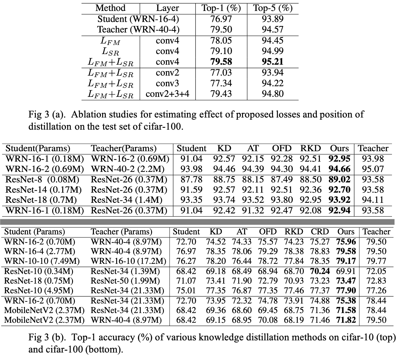
4. Experiment Results

Reference

Yang, Jing, et al. "Knowledge distillation via softmax regression representation learning." International Conference on Learning Representations. 2020.

Github Code: Knowledge Distillation via Softmax Regression Representation Learning