1. Data-free Knowledge distillation
Knowledge distillation: Dealing with the problem of training a smaller model (Student) from a high capacity source model (Teacher) so as to retain most of its performance.
As the word itself, We perform knowledge distillation when there is no original dataset on which the Teacher network has been trained. It is because, in real-world, most datasets are proprietary and not shared publicly due to privacy or confidentiality concerns.
In order to perform data-free knowledge distillation, it is necessary to reconstruct a dataset for training Student network. Thus, in Zero-Shot Knowledge Transfer via Adversarial Belief Matching, we train an adversarial generator to search for images on which the student poorly matches the teacher, and then use them to train the student.
2. Zero-shot knowledge transfer
2.1 Problem definition
- Teacher network: \(T(x)\) with an input image \(x\)
- Probability vector of teacher network: \(t\)
- Student network: \(S(x; \theta)\) with weigths \(\theta\)
- Probability vector of student network: \(s\)
- Generator: \(G(z; \phi) \) with weights \(\phi\)
- Pseudo data: \(x_p\) from a noise vector \(z \sim \mathcal{N} (0, I) \)
2.2 Method
The goal is to produce pseudo data from generator and use them to train student network by knowledge distillation.
To do this, Our zero-shot training algorithm is described in Algorithm 1. For \(N\) iterations we sample one batch of \(z\), and take \(n_G\) gradient updates on the generator whi learning rate \(\eta\), such that it produces pseudo samples \(x_p\) that maximize \(D_{KL} (T(x_p) || S(x_p))\).
\(D_{KL} (T(x_p) | | S(x_p))= \sum_i t_p^{(i)} log (t^{(i)}_p / s^{(i)}_p)\): Kullback-Leibler (KL) divergence between outputs of the teacher and student netowkrs on pseudo data (\(i\) is image classes)
| If maximize \(D_{KL} (T(x_p) | | S(x_p))\) \(\rightarrow\) \( t_p^{(i)}\) \(\uparrow\), \( \; s^{(i)}_p\) \(\downarrow\) |
| Elif minimize \(D_{KL} (T(x_p) | | S(x_p))\) \(\rightarrow\) \( t_p^{(i)}\) \(\downarrow\), \( \; s^{(i)}_p\) \(\uparrow\) |
We then take \(n_S\) gradient steps on the student with \(x_p\) fixed, such that it matches the teacher's predictions on \(x_p\). In practice, we use \(n_S > n_G\), which gives more time to the student to match the teacher on \(x_p\) and encourages the generator to explore other regions of the input space at the next iteration.
2.2 Extra loss functions
The high student entropy is a vital component of our method since it makes it hard for the generator to fool the student easily. Then, since many student-teacher pairs have similar block structures, we can add an attention term to the student loss as follows:
\[
L_s=D_{KL} (T(x_p) || S(x_p)) + \beta \sum_l^{N_L} \Vert \frac{f (A^{(t)}_l)}{ \Vert f (A^{(t)}_l) \Vert_2} - \frac{f (A^{(s)}_l)}{ \Vert f (A^{(s)}_l) \Vert_2}\Vert_2. \quad \cdots Eq. (1)
\]
- Hyperparameter: \(\beta\)
- Total layers: \(N_L\)
- Teacher and student activation blocks: \(A^{(t)}_l\) and \(A^{(s)}_l\) for layer \(l\)
- Total channels of l-th layer: \(N_{A_l}\)
- Spatial attention map: \(f(A_l)= \frac{1}{N_{A_l}} \sum_c a^2_{lc }\)
- We take the sum over some subset of \(N_L\) layers. The second term encourages both spatial attention maps between teacher and student networks to be similar. We don't use attention to the generator loss because it makes it too easy to fool the student. The training procedure is described in Fig. 1.

2.3 Toy experiment
The dynamics of our algorithm are illustrated in Fig. 2, where we use two layers MLPs for both teacher and student, and learn the pseudo points directly. These are initialized away from the real data manifold.
During training, pseudo points can be seen to explore the input space, typically running along decision boundaries where the student is most likely to match the teacher poorly. At the same time, the student is trained to match the teacher on the pseudo points, and so they must keep changing locations. When the decision boundaries between student and teacher are well aligned, some pseudo points will naturally depart from them and search for new high teacher mismatch regions, which allows disconnected decision boundaries to be explored as well.

3. Experiments & Results
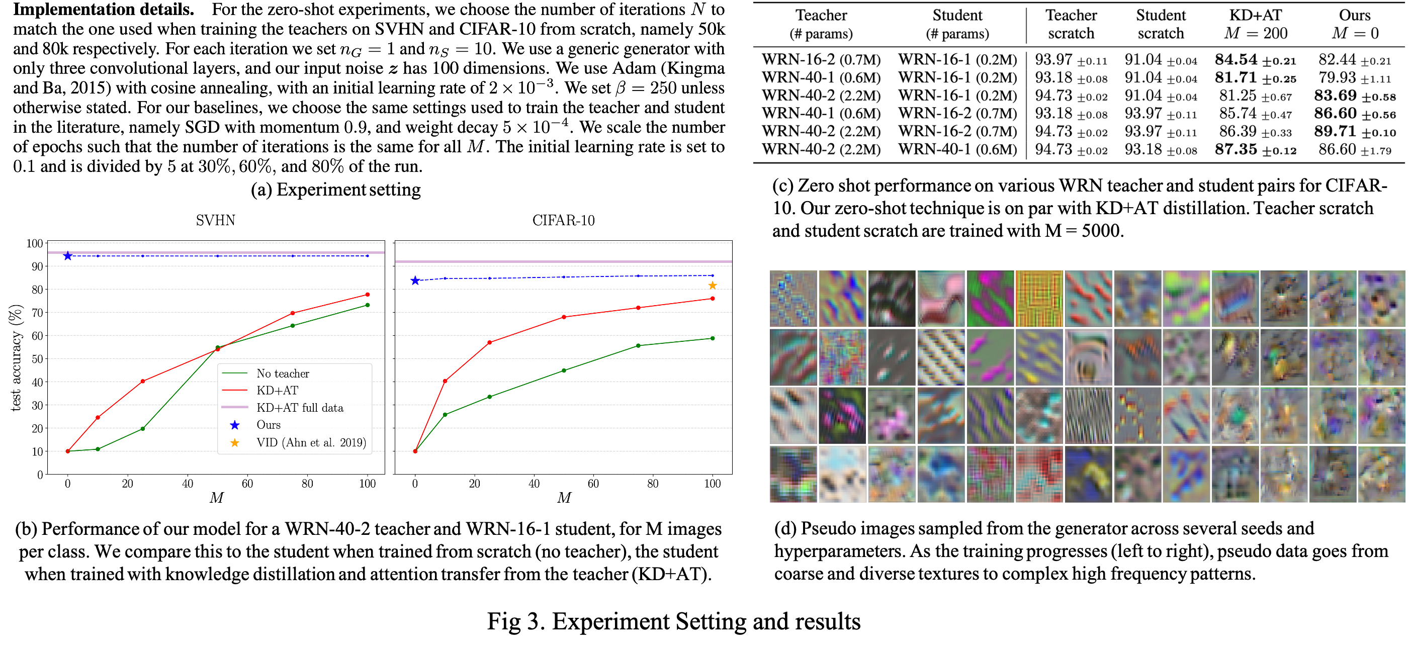
For each experiment, we run three seeds and report the mean with one standard deviation. The experiment setting is described in Fig. 3 (a).
3.1 CIFAR-10 and SVHN
We focus our experiments on two common datasets, SVHN and CIFAR-10. For both datasets, we use WideResNet (WRN) architecture. Our distillation results are shown in Fig. 3 (b). We include the few-shot performance of our method as a comparison, by naively finetuning our zero-shot model with \(M\) samples per class. Our method reaches 83.69 \(\pm\) 0.58% without using any real data, and increases to 85.91 \(\pm\) 0.24% when finetuned with \(M=100\) images per class.
3.2 Architecture dependence
We observe that some teacher-student pairs tend to work better than others, as in the case of few-shot distillation. The comparison results are shown in Fig. 3 (c). In zero-shot, deep students with more parameters don't necessarily help: the WRN-40-2 teacher distills 3.1% better to WRN-16-2 than to WRN-40-1, even though WRN-16-2 has less than half number of layers and a similar parameter count than WRN-40-1.
3.3 Nature of the pseudo data
Samples from the generator during training are shown in Fig. 3 (d). We notice that early in training the samples look like coarse textures and are reasonably diverse. After about 10% of the training run, most images produced by generator look like high-frequency patterns that have little meaning to humans.

3.4 Measuring belief match near decision boundaries
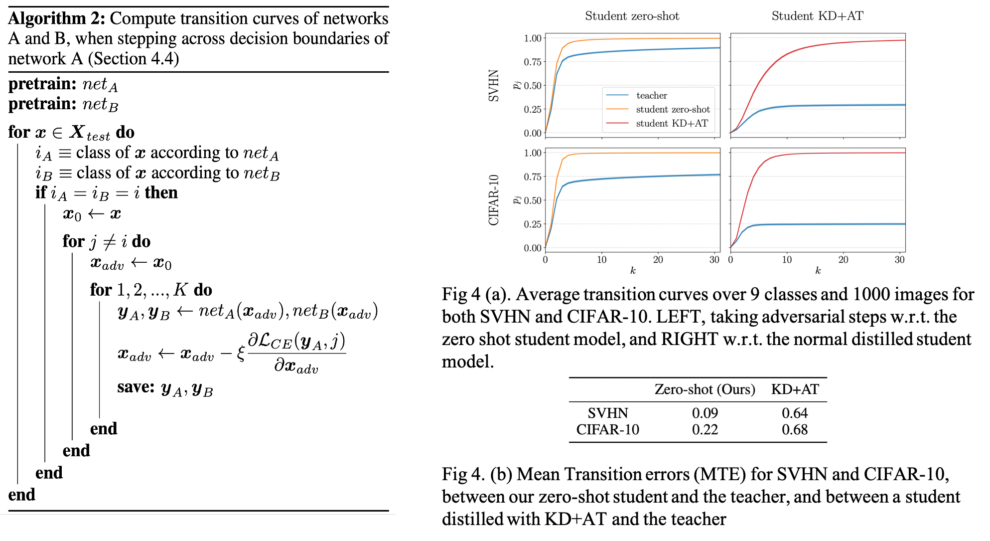
We would like to verify that the student is implicitly trained to match the teacher's predictions close to decision boundaries. For this, in Algorithm 2, we propose a way to probe the difference between beliefs of network \(A\) and \(B\) near the decision boundaries of \(A\). The procedure of Algorithm 2 is as follows.
- Sampling a real image: \(x\) from the test set \(X_{test}\) such that network \(A\) and \(B\) both give the same class prediction \(i\).
- For each class \(j \neq i\) we update \(x\) by taking \(K\) adversarial steps on network \(A\), with learning rate \(\xi\), to go from class $i$ to class $j$.
- The probability \(p^A_i\) of \(x\) belonging to class \(i\) according to network \(A\) quickly reduces, with a concurrent increase in \(p^A_j\).
- During 3. of process, we also record \(p^B_j\) and compare \(p^A_j\) ad \(p^B_j\).
Consequently, we are asking the following question, as we perturb \(x\) to move from class \(i\) to \(j\) according to network \(A\), to what degree do we also move from class \(i\) to \(j\) according to network \(B\)?
We refer to \(p_j\) curves as transition curves. For a dataset of \(C\) classes, we obtain \(C-1\) transition curves for each image \(x \in X_{test}\), and for each network \(A\) and \(B\). We show the average transition curves in Fig. 4 (a), in the case where network \(B\) is the teacher, and network \(A\) is either our zero-shot student or a standard student distilled with KD+AT.
The result is particularly surprising because while updating images to move from class \(i\) to class \(j\) on zero-shot student also corresponds to moving from class \(i\) to class \(j\) according to the teacher, the KD+AT student has flat \(p_j=0\) curves for several images even though KD+AT student was trained on real data, and the transition curves are also calculated for real data.
We can more explicitly quantify the belief match between networks \(A\) and \(B\) as we take steps to cross the decision boundaries of network \(A\). We define the Mean Transition Error (MTE) as the absolute probability difference between \(p^A_j\) and \(p^B_j\), averaged over \(K\) steps, \(N_{test}\) test images and \(C-1\) classes:
\[
MTE(net_A, net_B)= \frac{1}{N_{test}} \sum^{N_{test}}_n \frac{1}{C-1} \sum^{C-1}_c \frac{1}{K} \sum^K_k \vert p^A_j- p^B_j\vert \quad \cdots Eq. (2)
\]
The mean transition errors are reported in Fig. 4 (b).

Reference
Micaelli, Paul, and Amos J. Storkey. "Zero-shot knowledge transfer via adversarial belief matching." Advances in Neural Information Processing Systems 32 (2019).
'AI paper review > Model Compression' 카테고리의 다른 글
| EagleEye: Fast Sub-net Evaluation for Efficient Neural Network Pruning (0) | 2022.03.10 |
|---|---|
| Data-Free Knowledge Amalgamation via Group-Stack Dual-GAN (0) | 2022.03.09 |
| Dreaming to Distill Data-free Knowledge Transfer via DeepInversion (0) | 2022.03.09 |
| Data-Free Learning of Student Networks (0) | 2022.03.08 |
| Zero-Shot Knowledge Distillation in Deep Networks (0) | 2022.03.08 |
